A Book Recommendation System
Visualisations, analysis and a collaborative-filtering based recommendation system (in Python3), built using k-Nearest Neighbours and Matrix Factorisation approaches
To really understand the impact of recommendation systems, here is an extract from the book ‘The Long Tail ’ by Chris Anderson: “In 1988, a British mountain climber named Joe Simpson wrote a book called ‘Touching the Void’, a harrowing account of near death in the Peruvian Andes. It got good reviews but, only a modest success, it was soon forgotten. Then, a decade later, a strange thing happened. Jon Krakauer wrote ‘Into Thin Air’, another book about a mountain-climbing tragedy, which became a publishing sensation. Suddenly ‘Touching the Void’ started to sell again”.
The above effect was evidently a result of Amazon recommending ‘Touching the Void’ since it was based on the same theme (content-based recommendation). ‘Touching the Void’ eventually outsold ‘Into Thin Air’. This is the power of recommendation systems.
This article will demonstrate a collaborative filtering based approach, which is a really good starting point for any recommendation system. If collaborative filtering is something unfamiliar to you, you check out this article I have written on it: https://prianjali98.medium.com/recommender-systems-know-your-users-better-than-they-know-themselves-4568eef3d4ad . But as a quick recap, collaborative filtering based approaches recommend items based on users’ past behaviour. So two users are considered to be ‘similar’ if they have liked similar items in the past.
This project was done using the ‘goodreads-10k’ dataset which can be found here: https://www.kaggle.com/zygmunt/goodbooks-10k.
Importing the data
import pandas as pd
ratings = pd.read_csv('ratings.csv')
print(ratings.shape)
ratings.head()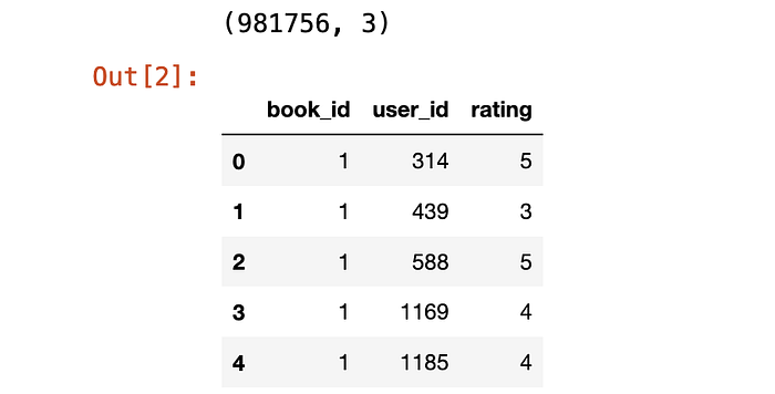
books = pd.read_csv('books.csv')
books.head()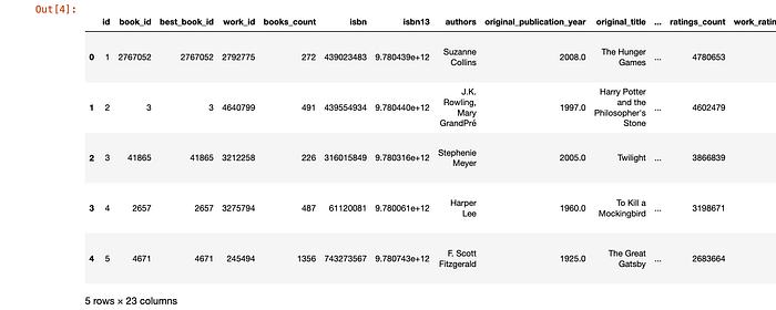
Cleaning the data
The first (and one of the most important steps) in building any machine learning model is cleaning the data. I started by dropping duplicates and rows with NaN values. In addition, I dropped some columns from the ‘books’ table which I won’t be using in building the model.
# Drop duplicates from ratings table
ratings.drop_duplicates(["user_id","book_id"], inplace = True) # Drop unwanted columns
books = books.drop(['best_book_id', 'work_id', 'books_count', 'isbn', 'isbn13', 'language_code', 'work_ratings_count', 'work_text_reviews_count', 'image_url', 'small_image_url', 'ratings_1', 'ratings_2', 'ratings_3', 'ratings_4', 'ratings_5'], axis=1, errors='ignore')# Drop duplicates from books table
books.drop_duplicates('title', inplace=True)# Find rows with NaN values and drop them from both tables
books_with_nan = books.isnull().any(axis=1)
for index, row in books[books_with_nan].iterrows():
    ratings = ratings[ratings.book_id != row.book_id]books.dropna(subset=['original_title'], inplace=True)
books.shape
Data Analysis and Visualization
We can find the top 10 most rated books and top 10 most popular books by analyzing the data in the ‘books’ table.
# Top 10 most rated books
top_rated = books.sort_values(by='ratings_count', ascending=False)
top_rated.head(10)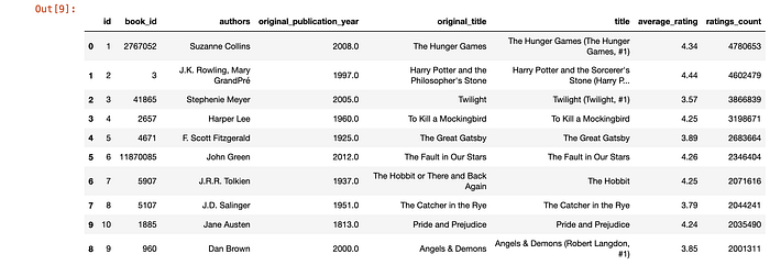
# Top 10 most popular books
popular = books.sort_values(by='average_rating', ascending=False)
popular.head(10)
Preparing the data
We will now need to merge the ‘books’ and ‘ratings’ table (along the common column — book_id).
books = books[['id', 'original_title']]
books = books.rename(columns={'id':'book_id'})
ratings_df = ratings.merge(books)
ratings_df = ratings_df.rename(columns={'original_title':'title'})
ratings_df.head()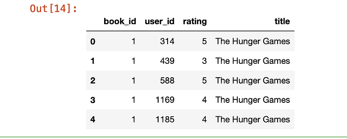
Pearson’s Correlation
Pearson Correlation is one of the most popular similarity measures for a Collaborative filtering based recommender system, to evaluate how much two users (user-based CF) or two items (item-based CF) are correlated.
# Creating a spreadsheet-style table indexed by user IDs, where each row is the rating given to a book by that user
book_mat = ratings_df.pivot_table(index ='user_id', columns = 'title', values = 'rating')
book_mat.fillna(0, inplace=True)
book_mat.head()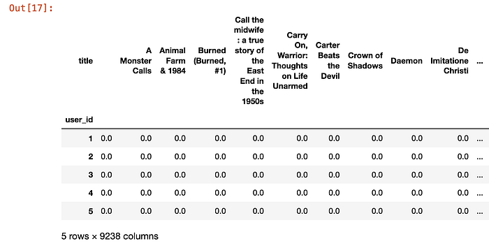
# Find books which are similar to 'The Hunger Games'
hunger_games_user_ratings = book_mat['The Hunger Games']
similar_to_hunger_games = book_mat.corrwith(hunger_games_user_ratings)
corr_hunger_games = pd.DataFrame(similar_to_hunger_games, columns = ['Correlation']).dropna()
corr_hunger_games.sort_values(by='Correlation', ascending=False).head(10)
While correlation-based prediction schemes are shown to perform well, they suffer from some limitations.
Removing noise
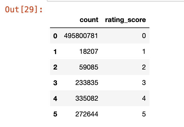
On carrying out some data analysis, we come to know that most books are not rated at all or are rated 0.
# Find the number of users and number of books
num_users = len(ratings_df.user_id.unique())
num_items = len(ratings_df.book_id.unique())# Find the number of books rated 0 or not rated
expected_number_ratings = num_users * num_items
zero_ratings_count = expected_number_ratings - ratings_df.shape[0]df_ratings_cnt_tmp = pd.DataFrame(ratings_df.groupby('rating').size(), columns=['count'])
top_row = pd.DataFrame({'count': zero_ratings_count}, index=[0])
df_ratings_cnt = pd.concat([top_row, df_ratings_cnt_tmp]).reset_index(drop = True)df_ratings_cnt['rating_score'] = df_ratings_cnt.index
df_ratings_cnt.reset_index(drop=True)
import matplotlib.pyplot as plt
fig = plt.figure()
ax = fig.add_axes([0,0,1,1])
ax.bar(df_ratings_cnt['rating_score'], df_ratings_cnt['count'], log=True)
ax.set_xlabel("Book Rating score")
ax.set_ylabel("Number of Ratings")
ax.set_title("Count vs Book Rating Score (in log scale)")
plt.show()
In order to remove the possibility of outliers and really understand preferences, we would need to remove books that have been rated less than 60 times and remove users who have rated less than 50 books.
df_books_cnt = pd.DataFrame(ratings_df.groupby('book_id').size(), columns=['count'])
popularity_threshold = 60
popular_books = list(df_books_cnt[df_books_cnt['count'] >= popularity_threshold].index)
df_filtered = ratings_df[ratings_df.book_id.isin(popular_books)]df_users_cnt = pd.DataFrame(ratings_df.groupby('user_id').size(), columns=['count'])
inactivity_threshold = 50
active_users = list(df_users_cnt[df_users_cnt['count'] >= inactivity_threshold].index)
df_filtered = df_filtered[df_filtered.user_id.isin(active_users)]
After removing unpopular movies and inactive users, now we are ready to fit a model using k-nearest neighbours.
Fitting a model using k-Nearest Neighbours algorithm
KNN is a simple, but popular supervised machine learning algorithm. The learning strategy in a KNN is more like memorization. It’s just like remembering what the answer should be when the question has certain characteristics (based on circumstances or past examples) rather than really knowing the answer. In a sense, KNN is often defined as a lazy algorithm because no real learning is done at the training time, just data recording.
To begin with, we create a Compressed Sparse Row (CSR) matrix, which helps in realizing substantial memory requirement reductions.
book_user_mat = df_filtered.pivot(index='book_id', columns='user_id', values='rating').fillna(0)
book_user_mat_sparse = csr_matrix(book_user_mat.values)
Next, we make use of sklearn’s NearestNeighbours library to fit the model.
from sklearn.neighbors import NearestNeighborsmodel_knn = NearestNeighbors(metric='cosine', algorithm='brute', n_neighbors=20, n_jobs=-1)
model_knn.fit(book_user_mat_sparse)
Being a lazy algorithm implies that KNN is quite fast at training but very slow at predicting. (Most of the searching activities and calculations on the neighbours is done at that time). It also implies that the algorithm is quite memory intensive because you have to store your dataset in memory (which means that there’s a limit to possible applications when dealing with big data).
Further, KNN is an algorithm that’s sensitive to outliers, causing predictions to become erratic. This makes data cleaning extremely important. Running a K-means first can help to identify outliers gathered into groups of their own. Also, keeping the neighbourhood large can help minimize the problem at the expense of a lower fit to the data (more bias than overfitting).
Making recommendations
In order to start making recommendation, I defined two functions — one to find matches in our data for the input book and the other to make the recommendations.
fuzzywuzzy is a library used for fuzzy matching — a technique used to find matches that may be less than 100% perfect.
from fuzzywuzzy import fuzzdef find_matches(input_book):
    matches = []
    for index, row in books.iterrows():
        ratio = fuzz.ratio(row.original_title.lower(), input_book.lower())
        if ratio >= 65:
            matches.append((row.original_title, index, ratio))
    matches = sorted(matches, key=lambda x: x[2])[::-1]
    if not matches:
        print('No match found')
        return
    print('Found possible matches: {0}\n'.format([x[0] for x in matches]))
    return matches[0][1]
Using the ‘fastai’ library to build a model that performs Matrix Factorisation
Matrix factorization is a simple embedding model, and has been found to be the most accurate approach to address the problem of high levels of sparsity. Matrix factorization techniques are usually more effective because they allow us to discover the latent features underlying the interactions between users and items.
To explore fastai, refer to this book: Deep Learning for Coders with fastai and PyTorch by Jeremy Howard and Sylvain Gugger
from fastai.collab import *
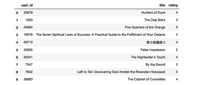
from fastai.tabular.all import *dls = CollabDataLoaders.from_df(ratings_df, user_name='user_id', item_name='title', bs=64)
dls.show_batch()
n_users  = len(dls.classes['user_id'])
n_books = len(dls.classes['title'])print('No. of users ', n_users)
print('No. of books ', n_books)

class DotProduct(Module):
    def __init__(self, n_users, n_books, n_factors):
        self.user_factors = Embedding(n_users, n_factors)
        self.book_factors = Embedding(n_books, n_factors)

    def forward(self, x):
        users = self.user_factors(x[:,0])
        books = self.book_factors(x[:,1])
        return (users * books).sum(dim=1)model = DotProduct(n_users, n_books, 50)
learn = Learner(dls, model, loss_func=MSELossFlat())
learn.fit_one_cycle(5, 5e-3)
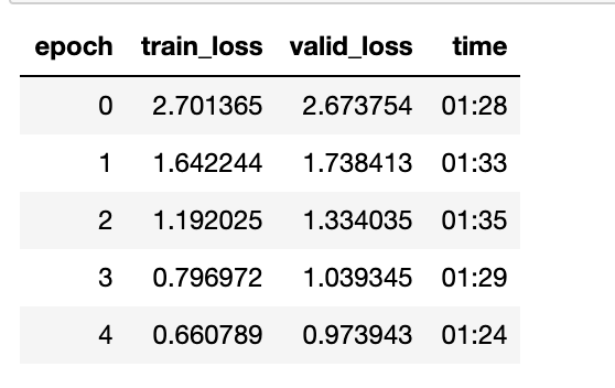
The first thing we can do to make this model a little bit better is forcing those predictions to be between 0 and 5. For this, we need to use a fastai method called ‘sigmoid_range’.
# Providing a range for y
class DotProduct(Module):
    def __init__(self, n_users, n_books, n_factors, y_range=(0,5.5)):
        self.user_factors = Embedding(n_users, n_factors)
        self.book_factors = Embedding(n_books, n_factors)
        self.y_range = y_range

    def forward(self, x):
        users = self.user_factors(x[:,0])
        books = self.book_factors(x[:,1])
        return sigmoid_range((users * books).sum(dim=1), *self.y_range)model = DotProduct(n_users, n_books, 50)
learn = Learner(dls, model, loss_func=MSELossFlat())
learn.fit_one_cycle(5, 5e-3)

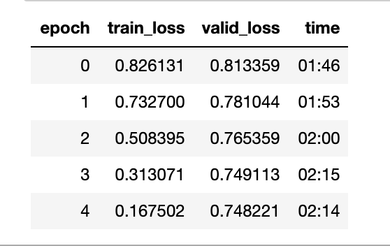
We can see that this model has weights, but what’s missing is the bias. We need to keep in mind that some users are just more positive or negative in their recommendations than others, and some movies are just plain better or worse than others. So, our model might do a little better by adding bias.
# Providing some bias
class DotProductBias(Module):
    def __init__(self, n_users, n_books, n_factors, y_range=(0,5.5)):
        self.user_factors = Embedding(n_users, n_factors)
        self.user_bias = Embedding(n_users, 1)
        self.book_factors = Embedding(n_books, n_factors)
        self.book_bias = Embedding(n_books, 1)
        self.y_range = y_range

    def forward(self, x):
        users = self.user_factors(x[:,0])
        books = self.book_factors(x[:,1])
        res = (users * books).sum(dim=1, keepdim=True)
        res += self.user_bias(x[:,0]) + self.book_bias(x[:,1])
        return sigmoid_range(res, *self.y_range)model = DotProductBias(n_users, n_books, 50)
learn = Learner(dls, model, loss_func=MSELossFlat())
learn.fit_one_cycle(5, 5e-3)
Conclusion
There are many steps that can be taken to improve the accuracy of this model. But this is a really good way to start building any recommender system. Exploring the different approaches to collaborative filtering was really insightful.
Please find the complete source code here:
https://github.com/chantal-rose/book_recommendation/blob/main/Book%20Recommendation.ipynb
